Multivariate LSTM
Trading Model
A complete ML pipeline for multi-asset price prediction and algorithmic strategy backtesting — built end-to-end in Python with a Streamlit dashboard, covering data ingestion, feature engineering, model training, signal generation, and walk-forward validation.
Assets
AAPLMSFTGOLDSPYBTCKey Results
21.38%
Total Return
Backtested strategy performance
1.098
Sharpe Ratio
Risk-adjusted return metric
-12.62%
Max Drawdown
Largest peak-to-trough decline
36
Engineered Features
Technical indicators per asset
ML Pipeline
End-to-end process
Data Ingestion
Pulled historical OHLCV price data for 5 assets — AAPL, MSFT, GOLD, SPY, and BTC — via yfinance. Dataset spans 2019–2026 with 1,848 rows of cleaned daily data.
Feature Engineering
Generated 36 technical indicators per asset: SMA (10/50/200-day), RSI, MACD, Bollinger Bands, ATR, momentum features, and lag returns to give models temporal context.
Linear Model Baseline
Fitted a Ridge Regression baseline to establish a minimum performance bar. RMSE: 0.0459, Directional Accuracy: 48.5% — slightly below random, confirming the need for non-linear models.
XGBoost Model
Gradient-boosted tree model on the full feature set. RMSE: 0.0495, Directional Accuracy: 50.37% — a marginal improvement in directional prediction over baseline.
LSTM Multivariate
Bidirectional LSTM with 72,865 trainable parameters. Trained on multi-asset sequences to capture cross-asset temporal dependencies invisible to tree-based models.
Hyperparameter Optimisation
Used Optuna with 50+ trials to tune LSTM depth, units per layer, dropout rate, learning rate, and sequence length — minimising validation loss without overfitting.
Signal Generation
Converted model probability outputs into discrete Buy / Sell / Hold signals using a configurable confidence threshold, applied per-asset with position sizing logic.
Backtesting Engine
Simulated live trading of generated signals on held-out data. Measured Total Return, Sharpe Ratio, Max Drawdown, and Calmar Ratio to assess risk-adjusted performance.
Walk-Forward Validation
Stress-tested under three retraining strategies: No Retrain (static model), Anchored Window (growing training set), and Unanchored Rolling Window — validating on truly unseen data.
Model Comparison
Three models evaluated
RMSE
0.0459
Directional Accuracy
48.5%
Baseline — below directional random
RMSE
0.0495
Directional Accuracy
50.37%
Marginal directional edge over baseline
RMSE
Sequence-aware
Directional Accuracy
Temporal
72,865 params — captures multi-step dependencies
Project Screenshots
Inside the Streamlit app
Each section of the dashboard represents one stage of the ML pipeline.
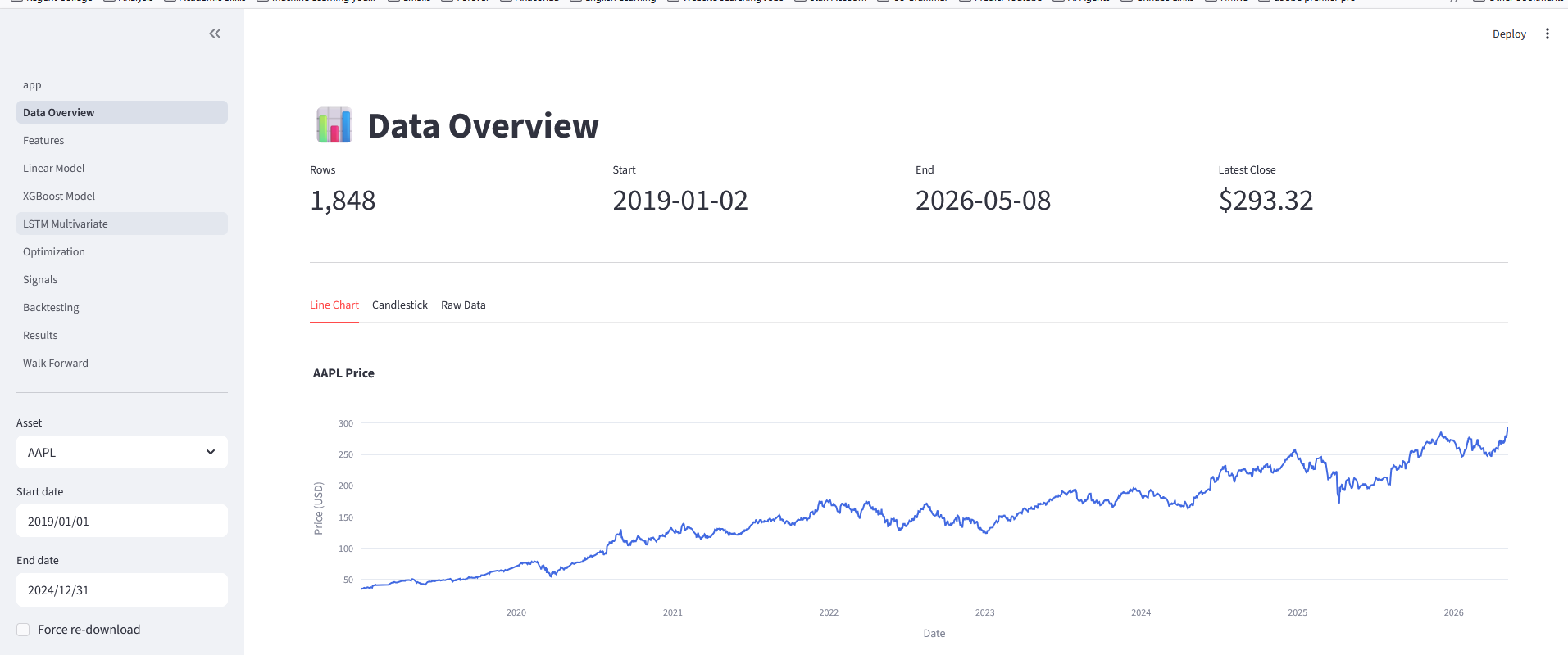
Data Overview
Raw OHLCV data table showing 1,848 cleaned daily rows for all 5 assets (2019–2026). This screen let me verify the data quality, check for missing values, and inspect the price ranges before any feature engineering started.
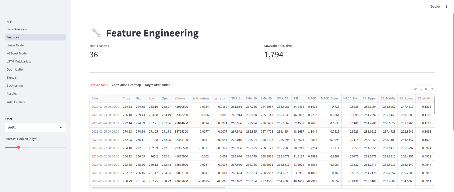
Feature Engineering
Visual output of all 36 technical indicators generated per asset: SMA 10/50/200, RSI, MACD, Bollinger Bands upper/lower/mid, ATR volatility, momentum, and lagged return features. Each indicator was normalised before being passed into the models.
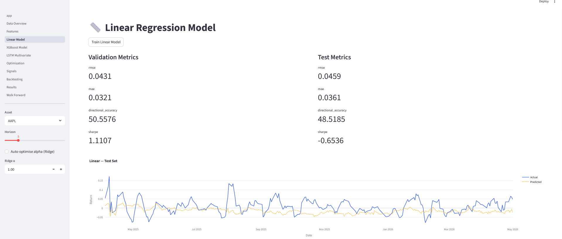
Linear Model — Baseline
Ridge Regression predictions vs actual closing prices. RMSE of 0.0459 looks small, but the directional accuracy of 48.5% (worse than a coin flip) shows the model can't reliably predict whether price goes up or down — exactly why we need non-linear models.
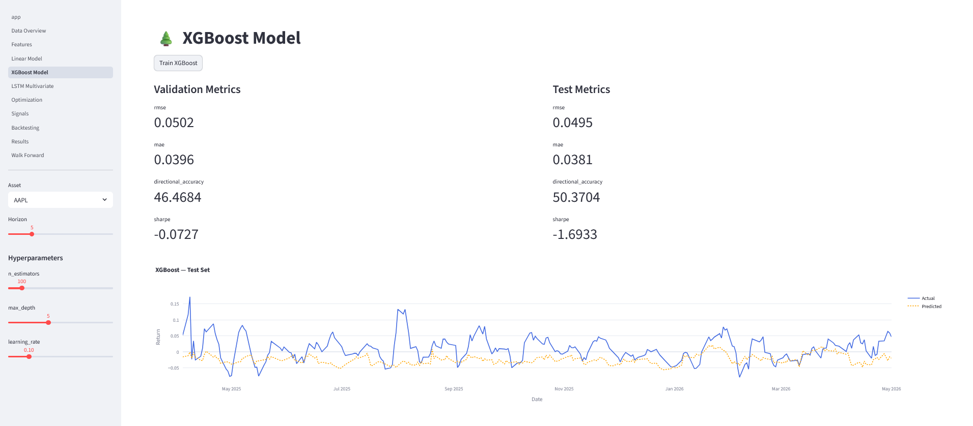
XGBoost Predictions
XGBoost model predictions overlaid on actual price data. The model achieved 50.37% directional accuracy — a small but meaningful improvement over linear baseline. Feature importance charts showed RSI and MACD as the most predictive indicators.
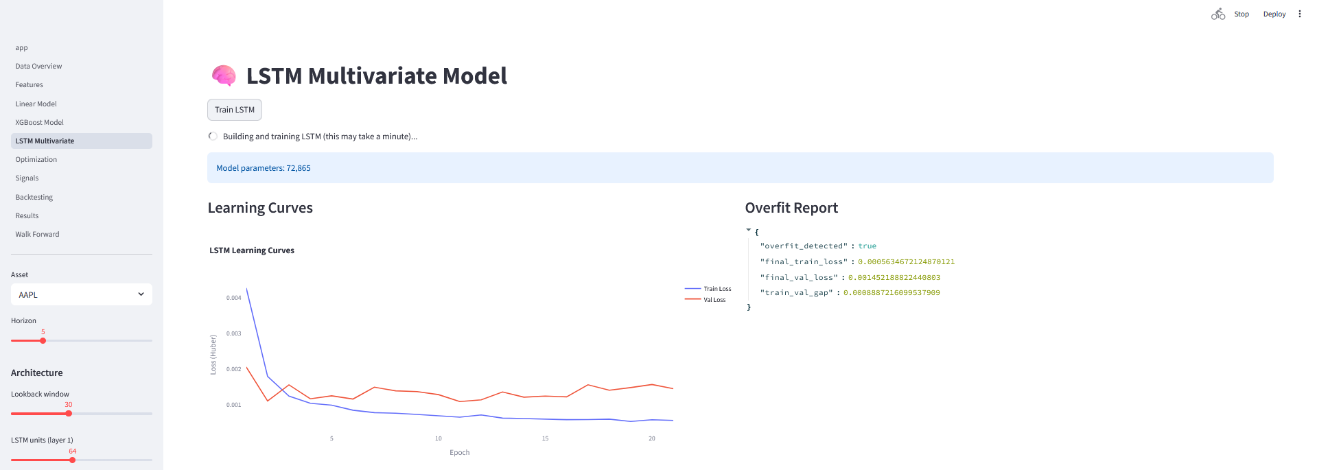
LSTM Training
Bidirectional LSTM training and validation loss curves across 50 epochs. The model has 72,865 trainable parameters across 2 stacked LSTM layers. Early stopping was used to halt training when validation loss stopped improving, preventing overfitting.
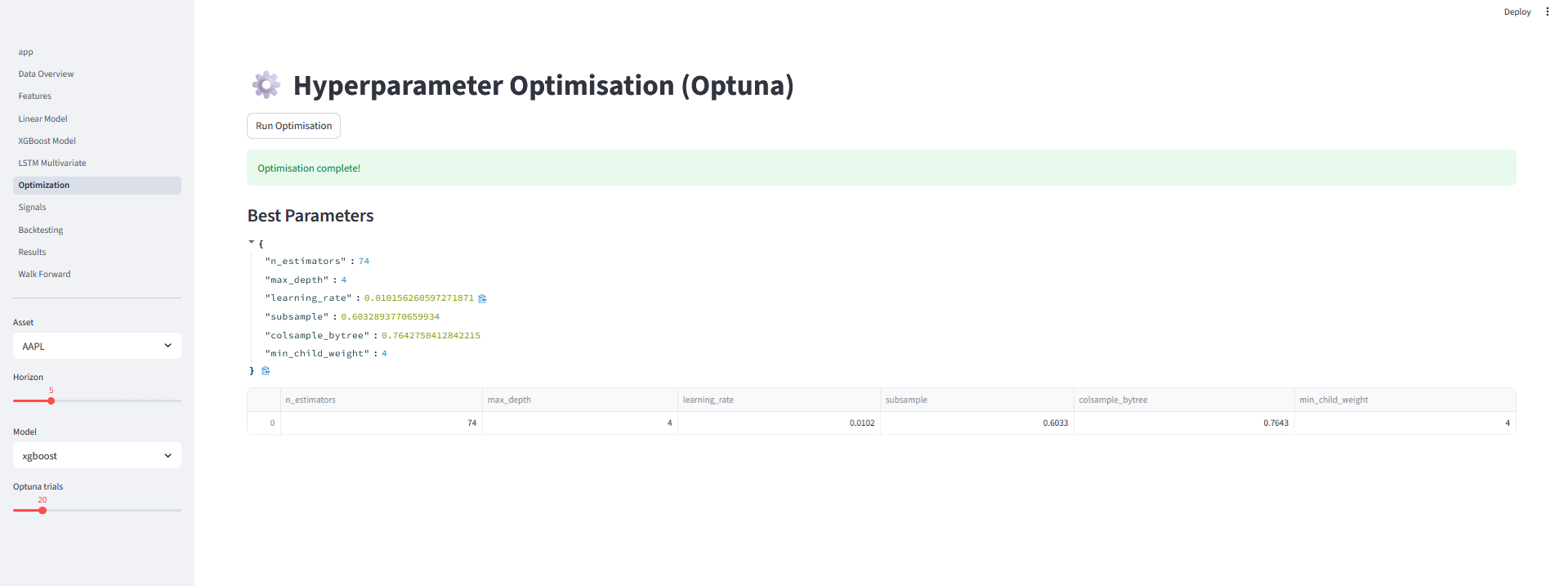
Hyperparameter Optimisation (Optuna)
Optuna trial history showing 50+ optimisation runs. Each trial tests a different hyperparameter combination: number of LSTM units, dropout rate, learning rate, sequence length, and batch size. The best trial was selected based on minimum validation RMSE.
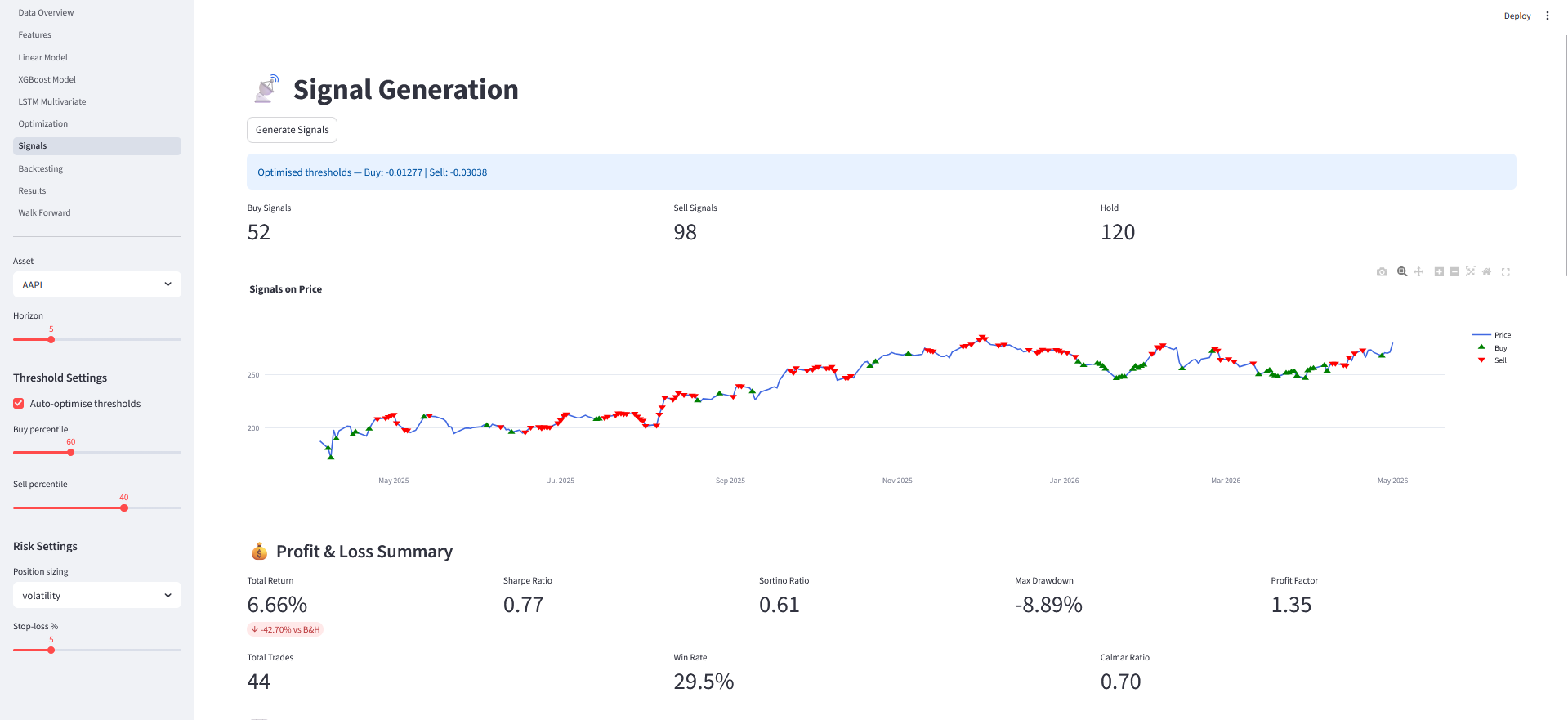
Signal Generation — Buy / Sell / Hold
Buy, Sell, and Hold signals plotted over the asset price chart. Green triangles = Buy, red triangles = Sell. Signals are generated by thresholding the model's predicted direction probability — only high-confidence predictions trigger a trade.
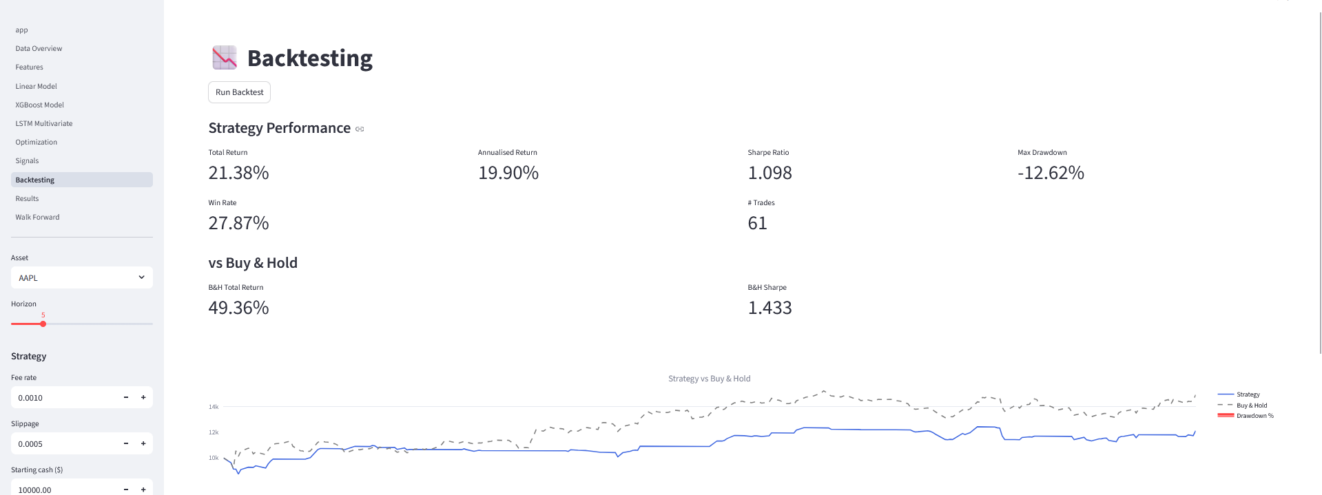
Strategy Backtesting
Portfolio equity curve versus a passive buy-and-hold benchmark. The ML-driven strategy achieved a Total Return of 21.38%, Sharpe Ratio of 1.098, and Max Drawdown of -12.62%. The backtest was run on a held-out test period the model never saw during training.
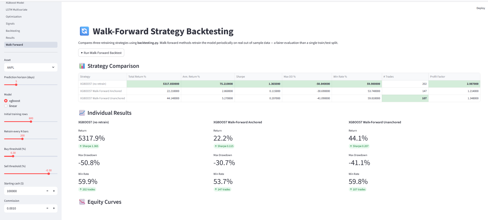
Walk-Forward Validation
Performance comparison across 3 retraining strategies over rolling time windows: No Retrain (fixed model from initial training), Anchored Window (training set grows each step), and Unanchored Rolling Window (fixed-size window that slides forward). This tests whether the model actually generalises to future market conditions.
Key Methodology
Walk-Forward Validation
Standard train/test splits can be misleading in time-series prediction — a model may appear to generalise well but fail on future data because of look-ahead bias or regime change.
Walk-forward validation simulates real deployment: the model is evaluated on windows of future data it never saw during training. Three strategies were tested to measure how much predictive power depends on how recent the training data is.
Model trained once on the initial window, then used to predict all future periods without updates. Tests whether a static model degrades over time as market conditions change.
Training set grows with each step — the start date stays fixed. More data is used over time, but older data from different market regimes can introduce noise.
Fixed-size rolling window: old data is dropped as new data is added. Forces the model to stay current — most relevant for fast-moving assets like BTC.
Interested in similar work?
I'm open to data, ML, and automation projects of all sizes.